tinygrad-notes

A complete trace: transpose → pad → add → reduce

All tutorials · Updated September 21, 2026 · tinygrad 8ad8f73

This walkthrough follows one computation through actual captured UOps and executed CPU and Metal programs. It is not a reconstruction of the old ShapeTracker pipeline. The captures use Python 3.14.6, BEAM=0, CPU arm64/ClangRenderer and METAL Apple7/MetalRenderer. The revision was checked against upstream when these notes were written; it is a reproducibility pin, not a promise that future tinygrad will produce identical graphs.

1. Establish the answer before looking at the compiler

from tinygrad import Tensor

x = Tensor([[1., 2., 3.], [4., 5., 6.]]).realize()
y = (x.T.pad(((1, 1), (1, 1))) + 10).sum(axis=1)
assert y.tolist() == [40., 45., 47., 49., 40.]
# Moving addition inside padding changes the meaning.
other = (x.T + 10).pad(((1, 1), (1, 1))).sum(axis=1)
assert other.tolist() == [0., 25., 27., 29., 0.]

The input is realized before tracing, so its initialization is not mistaken for part of the kernel under study. Transposition changes (2, 3) to (3, 2); padding changes that to (5, 4); reducing axis 1 leaves five elements.

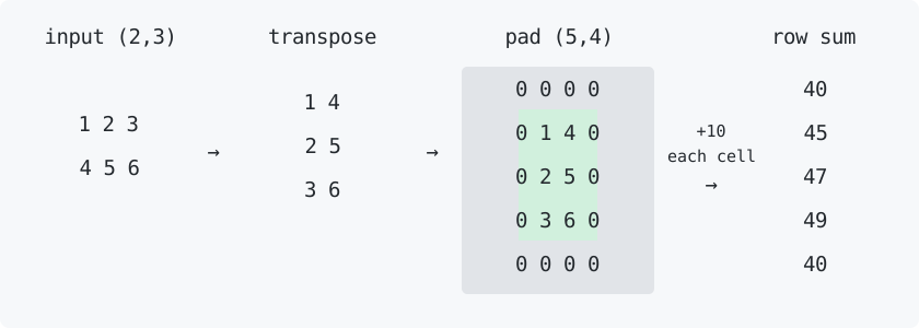
Coordinate and value diagram: transpose, zero padding, add ten, row reduction

The diagram is an explanatory drawing, not VIZ output. Here is the same arithmetic in text, before adding ten:

0 0 0  →  40
1 4 0  →  45
2 5 0  →  47
3 6 0  →  49
0 0 0  →  40

Each row receives four additions of ten. The zero-padded cells are real values in the expression, not permission to skip the later addition.

2. Tensor graph: movement is still explicit

Read the captured Tensor graph. Following its dependencies from the input gives BUFFER → RESHAPE → PERMUTE → PAD → ADD → PERMUTE → REDUCE (constants and shape operands omitted here).

Why two permutations? The first is our transpose. The second puts the reduced dimension first for the internal reduction representation. In this capture, REDUCE has arg=(Ops.ADD, 1): one leading dimension is reduced. That 1 is not simply the public axis=1 copied into the IR.

The internal PAD sources contain (1, 1) offsets and (5, 4) output dimensions. Do not read these as the public API’s ((before, after), ...) pairs.

3. Rangeification: derive the address and its validity

The prepared graph is the actual argument received by run_rangeify. Its returned graph uses explicit ranges, an indexed store, and an indexed input.

Call the output coordinate i, with 0 <= i < 5, and the reduction coordinate k, with 0 <= k < 4. Propagating coordinates backward:

Boundary	Coordinates or address
Padded tensor	`(i, k)`
Undo padding	`(i - 1, k - 1)`
Undo transpose	`(k - 1, i - 1)`
Flatten original `(2, 3)`	`3(k - 1) + (i - 1) = 3k + i - 4`

The coordinate is valid only when 1 <= i < 4 and 1 <= k < 3. The graph represents both an invalid-index sentinel and a zero-valued alternative. Its meaning can be summarized as:

valid = (1 <= i < 4) and (1 <= k < 3)
padded_value = input[3*k + i - 4] if valid else 0
output[i] = sum(padded_value + 10 for k in range(4))

This is explanatory pseudocode, not emitted source. In the capture, an inner WHERE selects the address or Invalid; an outer WHERE selects the indexed value or floating-point zero. Reading address -4 unconditionally and selecting zero afterward would not be an equivalent implementation.

The reduction now has arg=(Ops.ADD, 0) and an explicit reduction RANGE source. Range IDs can change in later transformations; follow dependencies and AxisType, not an assumed permanent axis number.

4. Schedule: one call, two buffers

The scheduled graph has one CALL in its outer LINEAR. Its kernel body is a SINK with STORE/END structure. The output parameter has five floats; the input parameter has six. The call supplies their buffer UOps.

There is no separately materialized 20-element padded tensor in this schedule. Its mapping and zero behavior are part of the consuming kernel. This is evidence about this pinned expression, not a rule that every transpose or padding operation always fuses.

For why other graphs need multiple calls and buffer-state ordering, see scheduling. Creating the schedule also updates Tensor references: the capture script executes the returned schedule before inspecting y.

5. Compiled CPU source: where did the loops go?

The complete generated CPU source loads input elements 0–3 as a float4 and elements 4–5 as a float2. Its stores compute:

output[0] = 40
output[1] = input[3] + input[0] + 40
output[2] = input[4] + input[1] + 40
output[3] = input[5] + input[2] + 40
output[4] = 40

These assignments paraphrase the generated vector store. The actual source has no for loop and no runtime padding predicate. The small fixed ranges have been expanded and simplified: the compiler can determine which lanes are padding and which six input elements are needed. It has not made padding irrelevant; its effect survives in the constants and selected input pairs.

Both loads stay within the six-element allocation. The first four outputs are written with a vector store, and the fifth separately. A different target, larger shape, or optimization configuration may retain loops or predicates. A RANGE in the scheduled graph is not a promise of a source-language loop.

6. The same computation on Metal

The Metal source uses device float*, Metal float4/float2 loads and .x/.y/.z/.w component access. It computes the same five expressions. The captured ProgramInfo and results report global and local sizes (1, 1, 1): this tiny program does not distribute five outputs across five threads. Its gid and lid parameters are unused.

That source was compiled and executed on Metal, not merely rendered. This establishes this example’s output on this device; it is not a benchmark, a tensor-core test, or evidence of scalable GPU utilization. Follow the Metal runtime chapter for compilation, binding, dispatch, and completion.

Reproduce and inspect the capture

From this notes repository, with Python 3.11+ and the pinned tinygrad checkout available:

PYTHONPATH=/path/to/tinygrad DEV=CPU python3 scripts/trace_movement.py /tmp/movement-cpu
PYTHONPATH=/path/to/tinygrad DEV=METAL python3 scripts/trace_movement.py /tmp/movement-metal

The second command requires a working Metal device. The script rejects a different revision or modified tracked tinygrad implementation, disables schedule-cache reuse, observes run_rangeify without replacing its result, compiles the actual schedule, executes it, and asserts the answer. It saves Tensor/prepared/rangeified/scheduled/program graphs, generated source, operation counts, and provenance. There is no separate stage 04 file: kernel splitting is reflected in stage 05, not independently instrumented.

CPU metadata and Metal metadata identify the captured targets. Generated binaries in program dumps are target-specific; do not expect byte-identical output across hosts. The regression examples below check semantics rather than matching source strings.

Challenge the mapping, not just the happy path

This independent Python oracle combines transpose, reversal, asymmetric padding, row broadcasting, and reduction. Sizes straddle common vector widths; inputs include negative values. None of the expected answers is computed with tinygrad.

from tinygrad import Tensor

for rows in (1, 2, 7):
  for cols in (1, 3, 31, 32, 33):
    data = [[float((r*7+c*3) % 19 - 9) for c in range(cols)] for r in range(rows)]
    # Transpose then reverse the new first axis; pad rows (2,1), columns (1,2).
    transformed = [[data[r][c] for r in range(rows)] for c in reversed(range(cols))]
    padded = [[0.]*(rows+3) for _ in range(2)]
    padded += [[0.] + row + [0., 0.] for row in transformed]
    padded += [[0.]*(rows+3)]
    bias = [float(i-2) for i in range(cols+3)]
    expected = [sum(v + b for v in row) for row, b in zip(padded, bias)]
    x = Tensor(data).realize()
    out = (x.T.flip(0).pad(((2, 1), (1, 2))) + Tensor(bias).reshape(-1, 1)).sum(axis=1)
    assert out.tolist() == expected, (rows, cols)
print("15 movement/broadcast/reduction cases passed")

These exact comparisons use small integer-valued floats whose sums are exactly representable. They do not establish arbitrary floating-point reassociation equivalence or cover empty dimensions, gradients, symbolic layouts, or every backend.

Implementation references: Tensor preparation, coordinate propagation, kernel splitting, codegen.